Efficiency of estimators

Suppose we want to estimate the mean $\theta$ of a normal distribution $\mathcal{N}(\theta, \sigma^2)$ from a sample of $n$ observations. What estimator should we use?

The most obvious candidate is the sample mean $T_{\text{mean}}$. However, there are other options. For instance, since the normal distribution is symmetric, the sample median $T_{\text{median}}$ is also an unbiased estimator of $\theta$, that is,

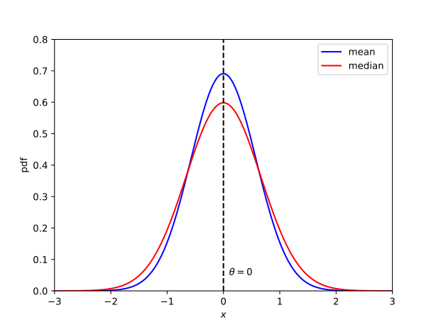
\[\mathbb{E}_\theta[T_{\text{mean}}]=\mathbb{E}_\theta[T_{\text{median}}]=\theta.\]

Should we therefore be indifferent between these two estimators? Not quite. Although both are centered at the true value $\theta$, they need not be equally concentrated around it. Intuitively, we would prefer the estimator with less spread. See Figure 1.

One way to quantify the spread around $\theta$ for an estimator $T$ is through its mean squared error

\[\operatorname{MSE}_\theta(T):=\mathbb{E}_\theta[(T-\theta)^2].\]

This quantity has a nice decomposition as a sum of variance and bias:

\[\operatorname{MSE}_\theta(T)=\operatorname{Var}_\theta(T)+(\mathbb{E}_\theta[T]-\theta)^2.\]

For an unbiased estimator, it thus simplifies to

\[\operatorname{MSE}_\theta(T)=\operatorname{Var}_\theta(T).\]

This suggests the following way of comparing estimators.

Definition. An estimator $T_1$ is more efficient than $T_2$ if

\[\operatorname{MSE}_\theta (T_1) \leq \operatorname{MSE}_\theta (T_2)\]

for all $\theta$, with strict inequality holding somewhere.

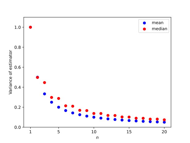
In our example, the sample mean is more efficient than the sample median. In fact, this holds for any sample size $n\geq 3$. See Figure 2. The variance of the sample mean is

\[\operatorname{Var}_\theta(T_{\text{mean}})=\dfrac{\sigma^2}{n},\]

whereas the variance of the sample median satisfies the asymptotic relation

\[\operatorname{Var}_\theta(T_{\text{median}})\approx\dfrac{\pi}{2}\dfrac{\sigma^2}{n}.\]

Therefore, asymptotically as $n\to \infty$, we get

\[\dfrac{\operatorname{Var}_\theta(T_{\text{median}})}{\operatorname{Var}_\theta(T_{\text{mean}})}\approx 1.57.\]

In other words, for large samples, the median needs about $57\%$ more observations to achieve the same variance as the mean.

However, the mean and median are just two choices among infinitely many unbiased estimators of $\theta$. For instance, since these distributions are symmmetric, we could take the average of the 10th and 90th sample percentiles. This raises two natural questions:

• Could we do better than the sample mean, that is, is there any unbiased estimator with smaller variance? Spoiler: no. For normal distributions, the sample mean is optimal.

• Is the mean always more efficient than the median? Spoiler: no. For some distributions, the sample median is actually more efficient.

Hopefully this is enough motivation to jump into the theory.

Information geometry

In our motivating example, we asked about the mean of the distribution. Of course, there is no reason to restrict our attention to this particular parameter. More generally, suppose we have a family of probability density functions

\[f_\theta:\Omega\to\mathbb R_{\geq 0}\]

parametrized by $\theta\in\Theta\subseteq\mathbb R^d$. Here, $\Omega$ is an arbitrary domain.

As a concrete example, consider the family of $1$-dimensional normal distributions $\mathcal{N}(\theta_1, \theta_2)$ with probability density functions

\[f_\theta(x)=\dfrac{1}{\sqrt{2\pi \theta_2}}\exp\left(-\dfrac{(x-\theta_1)^2}{2\theta_2}\right).\]

In this case, the domain is $\Omega=\mathbb{R}$, while the parameter space $\Theta$ is the upper half-plane $\mathbb{R}\times \mathbb{R}_+$, since $\theta_1$ is the mean and $\theta_2$ is the variance, which must be strictly positive.

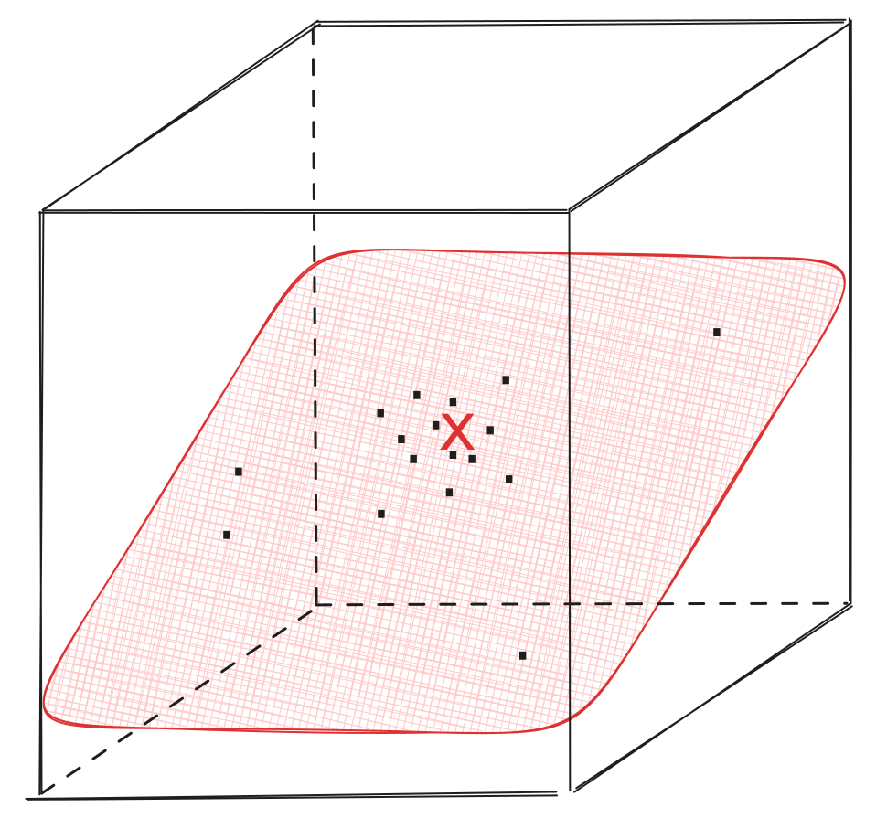
Each parameter value $\theta\in\Theta$ determines a unique probability density function $f_\theta$. Thus, we can think of the family $\lbrace f_\theta\rbrace_{\theta\in \Theta}$ as a $d$-dimensional surface inside the much larger, infinite-dimensional space of probability distributions on $\Omega$. Under suitable regularity assumptions, this surface forms a finite-dimensional manifold, called a statistical manifold. See Figure 3.

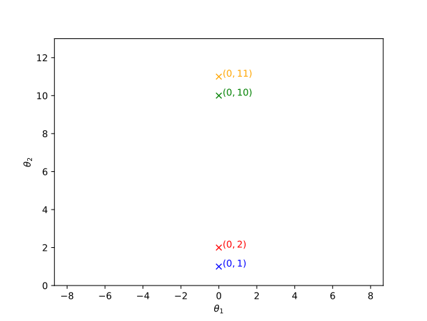
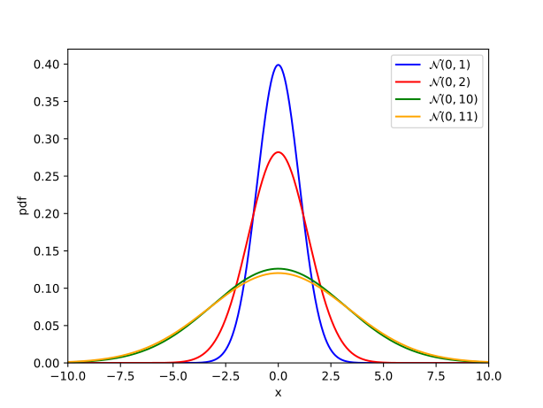
At first glance, it may seem that the parameter space $\Theta\subseteq\mathbb{R}^d$ already gives us everything we need. After all, it provides coordinates for the statistical manifold. But coordinates are not the same thing as geometry. In particular, the usual Euclidean distance between two parameter values need not reflect how different the corresponding probability distributions are. This distinction is illustrated heuristically in Figure 4.

What metric should we use on the statistical manifold parametrized by $\Theta$? In other words, how should we measure the distance between two probability distributions?

There are several ways to motivate the answer. One approach is to consider the relative difference between two probability density functions $f_\theta$ and $f_{\theta’}$ at a point $x\in \Omega$ where $f_\theta(x)>0$.:

\[\Delta_{\theta, \theta'} (x):= \frac{f_{\theta'}(x)}{f_\theta(x)} - 1.\]

When $\theta’$ is close to $\theta$ in parameter space, we can use the Taylor expansion

\[f_{\theta'}(x)=f_\theta(x)+\langle \nabla_\theta f_\theta(x), \theta'-\theta\rangle + \mathcal{O}(\Vert \theta'-\theta\Vert^2)\]

to obtain

\[\Delta_{\theta, \theta'} (x) =\langle \nabla_\theta \ln f_\theta(x), \theta'-\theta\rangle+ \mathcal{O}(\Vert \theta'-\theta\Vert^2).\]

The vector

\[s_\theta(x):= \nabla_\theta \ln f_\theta(x)\]

is called the score vector. Strictly speaking, $s_\theta(x)$ is a covector in $T^*_\theta \Theta$. It measures the infinitesimal change of the log-density in different parameter directions.

For instance, for a normal distribution $\mathcal{N}(\theta_1, \theta_2)$, a straightforward computation yields

\[s_\theta(x)=\left(\begin{matrix} \dfrac{x-\theta_1}{\theta_2} \\ -\dfrac{1}{2\theta_2}+\dfrac{(x-\theta_1)^2}{2\theta_2^2} \end{matrix}\right).\]

See Figure 5 to visualize these score vectors at different points of the parameter space.

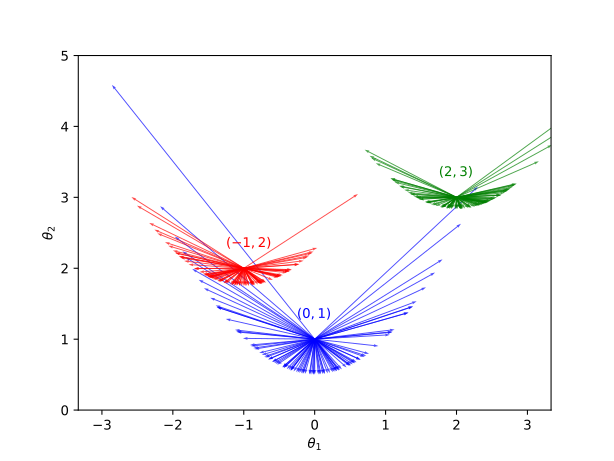
Since the score vector depends on the observation $x\in \Omega$, we cannot use it directly to define a tangent vector on the statistical manifold. One might try to average the score over all possible observations, but this does not work because the expected value is always zero:

\[\begin{aligned} \mathbb{E}_\theta[s_\theta] &=\int_{\Omega}f_\theta(x)s_\theta(x)\, dx\\ &=\int_{\Omega}f_\theta(x)\nabla_\theta \ln f_\theta(x)\, dx\\ &=\nabla_\theta\int_{\Omega}f_\theta(x)\, dx\\ &=0. \end{aligned}\]

Instead, given two tangent vectors $u, v\in T_\theta \Theta$, we define

\[g_\theta(u, v):=\mathbb{E}_\theta[\langle s_\theta , u\rangle \langle s_\theta , v\rangle].\]

This is the Fisher information metric on the statistical manifold. For nearby parameters $\theta’$ and $\theta$, our Taylor expansion gives

\[\begin{aligned}\mathbb{E}_\theta[\Delta_{\theta',\theta}^2]&=\mathbb{E}_\theta[\langle s_\theta, \theta'-\theta\rangle^2] + \mathcal{O}(\Vert \theta'-\theta\Vert^3)\\ &=g_\theta(\theta'-\theta, \theta'-\theta) + \mathcal{O}(\Vert \theta'-\theta\Vert^3). \end{aligned}\]

Thus, to second order, the Fisher information metric measures the squared infinitesimal relative distance between nearby probability distributions.

In coordinates, the metric can be represented by a matrix $I_\theta$ characterized by

\[g_\theta(u, v)=\langle u, I_\theta v\rangle.\]

Since the expected value of the score vector is zero, the matrix $I_\theta$ is nothing but its covariance matrix:

\[I_\theta = \operatorname{Cov}_\theta(s_\theta, s_\theta).\]

For instance, in our ongoing example, the Fisher information matrix is

\[I_\theta = \left(\begin{matrix} \frac{1}{\theta_2} & 0 \\ 0 & \frac{1}{2\theta_2^2} \\ \end{matrix}\right).\]

Equivalently, the expression for the Fisher metric is

\[ds^2_{\text{Fisher}}=\dfrac{d\theta_1^2}{\theta_2} + \dfrac{d\theta_2^2}{2\theta_2^2}.\]

Note that if we use coordinates $x:=\theta_1 / \sqrt{2}$ and $y:=\sqrt{\theta_2}$, we obtain a scalar multiple of the Poincaré metric in the hyperbolic upper half-plane:

\[ds^2_{\text{Fisher}}=2\dfrac{dx^2+dy^2}{y^2}.\]

Therefore, the Fisher distance $\rho_{\text{Fisher}}$ between $\theta$ and $\theta’$ can be expressed in terms of the Poincaré distance:

\[\rho_{\text{Fisher}}(\theta, \theta')=\sqrt{2}\rho_{\text{Poincaré}}\left(\dfrac{\theta_1}{\sqrt{2}}+i\sqrt{\theta_2}, \dfrac{\theta_1'}{\sqrt{2}}+i\sqrt{\theta_2'}\right).\]

We can visualize this in Figure 6.

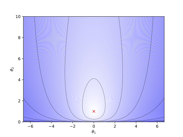
By introducing the notion of Fisher distance, we have formalized the observation from Figure 4 that the distributions $\mathcal N(0,10)$ and $\mathcal N(0,11)$ are much closer to each other than $\mathcal N(0,1)$ is to $\mathcal N(0,2)$.

Relation to the Kullback–Leibler divergence

We motivated the Fisher metric by considering the relative difference between two probability density functions $f_\theta$ and $f_{\theta’}$. Another approach is to derive it from the well-known Kullback–Leibler (KL) divergence, also known as relative entropy:

\[D_{\text{KL}}(f_\theta, f_{\theta'}):=\int_\Omega f_\theta(x)\ln \dfrac{f_\theta(x)}{f_{\theta'}(x)}\, dx.\]

Intuitively, the KL divergence measures the information lost when we use $f_{\theta’}$ to model data generated according to $f_\theta$. Although it quantifies the discrepancy between two distributions, it is not a genuine distance: it is generally asymmetric and does not satisfy the triangle inequality. Nevertheless, it is non-negative, with equality if and only if the two distributions agree almost everywhere.

Fix $\theta$ and consider the KL divergence as a function of $\theta’$. It attains its minimum at $\theta’=\theta$, where its value and gradient vanish. A second-order Taylor expansion around this point therefore gives

\[D_{\text{KL}}(f_\theta, f_{\theta'})=\dfrac{1}{2}\langle \theta'-\theta, H_\theta (\theta'-\theta)\rangle + \mathcal{O}(\Vert \theta-\theta'\Vert^3),\]

where $H_\theta$ is the Hessian matrix with respect to $\theta’$, evaluated at $\theta’=\theta$.

A quick calculation shows that $I_\theta=H_\theta$. In other words, the Fisher metric is the local quadratic approximation of the KL divergence.

Remarkably, this construction is not specific to the KL divergence. Under suitable regularity conditions, any notion of divergence satisfying the information monotonicity principle induces the Fisher metric, up to a constant factor, through its Hessians along the diagonal. In this sense, the Fisher metric is intrinsic to the statistical model: it endows the space of probability distributions with a natural geometry.

Cramér–Rao bound

Armed with this geometric viewpoint, we can return to our original question: given an unbiased estimator $T$ of a parameter $\theta$, can we find a non-trivial lower bound for $\operatorname{Var}_\theta(T)$?

The key insight is to apply the Cauchy–Schwarz inequality to the covariance between the estimator $T$ and the score vector $s_\theta$, combined with the fact that the covariance matrix of $s_\theta$ is the Fisher information matrix. Indeed, we have

\[\langle u , \operatorname{Cov}_\theta(T, s_\theta) v \rangle ^2 \leq \langle u, \operatorname{Var}_\theta (T) u\rangle \langle v, I_\theta v\rangle\]

for all for all tangent vectors $u, v\in T_\theta \Theta$.

For an arbitrary estimator $T$ of $\theta$, since the score vector $s_\theta$ has zero expectation, we have

\[\begin{aligned} \langle u,\operatorname{Cov}_\theta(T,s_\theta)v\rangle &=\mathbb E_\theta\left[ \langle u,T-\mathbb E_\theta[T]\rangle \langle s_\theta,v\rangle \right]\\ &=\mathbb E_\theta\left[ \langle u,T\rangle\langle s_\theta,v\rangle \right]\\ &=\int_\Omega f_\theta(x) \langle u,T(x)\rangle \langle s_\theta(x),v\rangle\, dx\\ &=\int_\Omega \langle u,T(x)\rangle \langle\nabla_\theta f_\theta(x),v\rangle\, dx\\ &=\left\langle u, D_\theta\mathbb E_\theta[T],v \right\rangle, \end{aligned}\]

where $D_\theta\mathbb{E}_\theta[T]$ denotes the Jacobian of the expectation of $T$ with respect to $\theta$. Since this holds for all $u$ and $v$, we obtain

\[\operatorname{Cov}_\theta(T,s_\theta)=D_\theta\mathbb E_\theta[T].\]

For an unbiased estimator, we get

\[\operatorname{Cov}_\theta(T,s_\theta)=I.\]

Consequently, for any non-zero $u\in T_\theta \Theta$, we can apply the inequality with $v=I_\theta^{-1}u$ to obtain

\[\begin{aligned} \langle u , \operatorname{Var}_\theta(T) u\rangle & \geq \frac{\langle u, I_\theta^{-1}u\rangle^2} {\langle I_\theta^{-1}u,I_\theta I_\theta^{-1}u\rangle}\\ & =\langle u, I_\theta^{-1}u\rangle. \end{aligned}\]

We conclude that

\[\operatorname{Var}_\theta(T)\succeq I_\theta^{-1}.\]

This is precisely the Cramér–Rao bound. The notation $A \succeq B$ means that the matrix $A-B$ is positive semidefinite.

The bound tells us that the more information the model carries about its parameters, the smaller the variance an unbiased estimator can potentially achieve. It gives us a fundamental lower limit on estimation error, regardless of the particular unbiased estimator used.

From one observation to a sample

Suppose $x_1, \ldots, x_n$ are i.i.d. observations drawn from a distribution $f_\theta$. By independence, the joint probability density is

\[f_\theta^{(n)}(x_1,\ldots,x_n) =\prod_{i=1}^n f_\theta(x_i).\]

Instead of considering the original statistical manifold

\[\{f_\theta \mid \theta\in \Theta\},\]

we can consider the statistical manifold of $n$ independent observations,

\[\{f_\theta^{(n)}\mid \theta \in \Theta\}.\]

The parameter space is still $\Theta$: we have not introduced $n$ independent parameters but rather $n$ observations governed by the same parameter $\theta$. The new domain is $\Omega^n$.

The score of the sample is the sum of the individual scores:

\[\begin{aligned} s_\theta^{(n)}(x_1, \ldots, x_n)&=\nabla_\theta\log f_\theta^{(n)}(x_1, \ldots, x_n)\\ &=\sum_{i=1}^n s_\theta(x_i). \end{aligned}\]

Since the individual scores are independent and have mean zero, the cross terms vanish when we take the expectation of the outer product. Consequently, the Fisher information metric on the sample model is

\[\begin{aligned} g_\theta^{(n)}(u,v) &=\mathbb E_\theta\left[ \langle s_\theta^{(n)},u\rangle \langle s_\theta^{(n)},v\rangle \right]\\ &=n\,g_\theta(u,v). \end{aligned}\]

Equivalently, the Fisher information matrix satisfies

\[I_\theta^{(n)}=nI_\theta.\]

Geometrically, the Fisher metric on the sample model is the original metric scaled by $n$. Thus, infinitesimal distances are scaled by $\sqrt{n}$: as the sample size increases, the statistical model becomes more informative about the underlying parameter.

We can now return to our original questions: can we find an unbiased estimator more efficient than the sample mean, and is the sample mean always more efficient than the sample median?

Consider first $n$ i.i.d. observations from a normal distribution $\mathcal N(\theta,\sigma^2)$, where $\sigma^2$ is known. The Cramér–Rao bound implies that any unbiased estimator $T$ of $\theta$ satisfies

\[\operatorname{Var}_\theta(T)\geq \frac{1}{I_\theta^{(n)}}=\frac{\sigma^2}{n}.\]

But the sample mean attains this bound, since

\[\operatorname{Var}_\theta(T_{\text{mean}})=\frac{\sigma^2}{n}.\]

Therefore, no unbiased estimator can have smaller variance than the sample mean in this setting. The sample mean is an efficient estimator of the normal distribution’s mean.

What about the second question? Is the sample mean always more efficient than the sample median?

Consider instead the Laplace distribution $\operatorname{Laplace}(\theta,b)$, with location parameter $\theta$ and scale parameter $b$. The sample mean has variance

\[\operatorname{Var}_\theta(T_{\text{mean}})=\frac{2b^2}{n}.\]

By contrast, the sample median has asymptotic variance

\[\operatorname{Var}_\theta(T_{\text{median}}) \approx\frac{b^2}{n}\]

as $n\to \infty$. Thus, for sufficiently large samples, the sample median is approximately twice as efficient as the sample mean. In this case, the Cramér-Rao bound happens to be $b^2/n$, so the median is asymptotically efficient.

This illustrates that the most efficient estimator depends on the Fisher geometry of the underlying statistical manifold.